Practical Guide: Building a Graphene Fiber Biosensor for Cancer Biomarker Detection

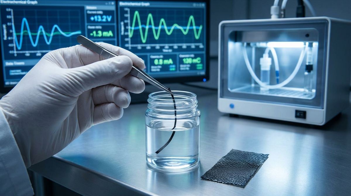
The ability to monitor biochemical processes in real-time within living tissue offers a revolutionary window into understanding disease. For cancer research, two molecules of immense interest are nitric oxide (NO) and hydrogen peroxide (H2O2). These reactive species play critical roles in tumor progression and cell signaling, but their fleeting nature and low concentrations make them incredibly difficult to measure simultaneously. Traditional methods often require sample extraction, which can alter concentrations and lose valuable temporal data.

This guide presents a practical approach to building an implantable, flexible electrochemical biosensor capable of this very task. Based on the work of Shanting Li and colleagues in their 2026 paper, "Implantable Graphene Fiber Sensor Functionalized with Enzyme-Mimicking Fe-Porphyrin for In Vivo Simultaneous Monitoring of NO and H2O2 in Cancer," we will walk through the fabrication and testing of a sensor that leverages the unique properties of graphene. The goal is to create a device that can provide continuous, in situ data, offering a more accurate picture of the tumor microenvironment. This project is a fantastic example of the advanced capabilities of modern graphene sensors and their growing importance in medicine.

Project Overview: What We Are Building

The final device is a freestanding, flexible microelectrode designed for implantation. Its core is a graphene fiber that has been chemically modified to enhance its electrical properties and surface area. This fiber acts as the conductive substrate.

The sensing capability comes from a specialized coating: a metal-organic framework (MOF) known as PCN-224(Fe). This iron-porphyrin MOF acts as an enzyme mimic, possessing catalytic sites that are highly active toward both NO and H2O2. This catalytic activity is what allows the sensor to detect the target molecules at extremely low concentrations.

When a specific voltage is applied, the MOF catalyzes the electrochemical reduction or oxidation of the target molecules at the graphene surface. This generates a measurable electrical current that is directly proportional to the concentration of the analyte. Because NO and H2O2 react at different electrochemical potentials, the sensor can distinguish between them and measure both simultaneously from a single electrode.

Materials and Equipment

This project involves chemical synthesis and electrochemical analysis. Ensure you have the proper personal protective equipment (PPE) and work in a well-ventilated area, preferably a fume hood.

Chemicals and Consumables

Graphene Oxide (GO) dispersion: A stable aqueous dispersion, typically 1-5 mg/mL. The quality of your starting GO is critical.
Boric Acid (H3BO3): For boron doping.
Hydrazine Hydrate (N2H4·H2O): A strong reducing agent. Handle with extreme caution.
Iron(III) Chloride (FeCl3): Metal source for the MOF.
Meso-tetra(4-carboxyphenyl)porphine (TCPP): The organic ligand for the MOF.
Benzoic Acid: A modulator for MOF synthesis.
N,N-Dimethylformamide (DMF): Solvent for MOF synthesis.
Ethanol and Acetone: For cleaning and rinsing.
Phosphate-Buffered Saline (PBS): For creating the testing electrolyte, typically pH 7.4 to mimic physiological conditions.
S-Nitroso-N-acetyl-DL-penicillamine (SNAP): A common NO donor for creating calibration standards.
Hydrogen Peroxide (H2O2): 30% solution for creating calibration standards.
Interfering species (for selectivity testing): Ascorbic acid, uric acid, glucose, dopamine.
High-purity Nitrogen or Argon gas: For creating an inert atmosphere during thermal annealing.
Deionized (DI) water.

Equipment

Electrochemical Workstation: A potentiostat capable of performing cyclic voltammetry (CV) and differential pulse voltammetry (DPV) or chronoamperometry.
Three-Electrode Cell: A glass cell to hold the electrolyte, with ports for the working, counter, and reference electrodes.
Working Electrode: Your fabricated graphene fiber sensor.
Reference Electrode: Silver/Silver Chloride (Ag/AgCl) is standard.
Counter Electrode: A platinum (Pt) wire or mesh.
Syringe Pump and Wet-Spinning Apparatus: For creating the graphene oxide fibers. This is specialized equipment; we will discuss alternatives.
Tube Furnace: Capable of reaching at least 800°C with atmospheric control.
Autoclave or Sealed Reaction Vessel: For the solvothermal synthesis of the MOF.
Sonicator: For dispersing materials.
Centrifuge: For washing and collecting synthesized MOF particles.
pH Meter.
Micropipettes.

Step-by-Step Fabrication Guide

This process is divided into three main stages: creating the doped graphene fiber substrate, synthesizing the catalytic MOF, and combining the two to form the final sensor.

Step 1: Prepare the Nitrogen and Boron Codoped Graphene Fiber

The foundation of the sensor is a highly conductive and flexible fiber. The source paper uses a custom wet-spinning process.

1. Prepare the Spinning Dope: Start with a concentrated GO aqueous dispersion (e.g., 10 mg/mL). Add boric acid to this dispersion. The paper does not specify the exact ratio, so a reasonable starting point based on similar literature would be a 10:1 mass ratio of GO to boric acid. Sonicate the mixture for 1-2 hours to ensure homogeneous dispersion.
2. Wet-Spinning: This is the most technically challenging step. The GO/boric acid dope is loaded into a syringe and extruded through a fine needle (e.g., 25-gauge) into a coagulation bath (typically an aqueous solution of a salt like CaCl2 or a solvent like ethanol). As the GO solution enters the bath, it solidifies into a continuous fiber. The fiber is drawn out of the bath and collected on a spool. The drawing speed and extrusion rate must be carefully controlled to achieve a uniform fiber diameter.
3. Chemical Reduction: Immerse the collected GO fibers in a solution of hydrazine hydrate. An engineering assumption would be to use a 1-2% solution and heat it to 80-95°C for several hours. This step reduces the oxygen-containing functional groups on the GO, improving electrical conductivity. The hydrazine also serves as a nitrogen source for N-doping. After reduction, thoroughly rinse the fibers with DI water and ethanol to remove residual reactants.
4. Thermal Annealing: Place the dried, reduced fibers into a tube furnace. Heat them under an inert atmosphere (argon or nitrogen). The source paper does not specify the exact temperature profile. A common protocol for this type of material is to ramp to 600-800°C and hold for 1-2 hours. This high-temperature step further reduces the graphene, facilitates the incorporation of boron and nitrogen into the carbon lattice, and improves the fiber's crystallinity and conductivity. Let the furnace cool to room temperature before removing the fibers.

You should now have black, flexible, and conductive N, B-codoped graphene fibers.

Step 2: Synthesize the PCN-224(Fe) MOF Catalyst

This solvothermal method creates the porous, crystalline structure that will serve as the catalytic sensor coating.

1. Prepare the Precursor Solution: In a glass vial, dissolve the porphyrin ligand (TCPP) and the metal salt (FeCl3) in DMF. The molar ratio is critical for proper crystal formation. Based on established protocols for PCN-224, a ratio of approximately 1:2 (TCPP:FeCl3) is a good starting point. Add benzoic acid as a modulator, which helps control crystal size and quality; a large excess (e.g., 30-50 equivalents relative to TCPP) is often used.
2. Solvothermal Reaction: Seal the vial in a Teflon-lined autoclave or a suitable pressure vessel. Heat the vessel in an oven. The paper does not provide the exact temperature and time. A typical condition for this synthesis is 120-150°C for 12-24 hours.
3. Purification: After the reaction, let the vessel cool to room temperature. You will see a dark-colored precipitate, which is the PCN-224(Fe) MOF. Collect the solid product by centrifugation. Wash it repeatedly with fresh DMF and then ethanol to remove any unreacted precursors trapped within the pores. Finally, dry the purified MOF powder in a vacuum oven at a mild temperature (e.g., 60-80°C).

Step 3: Functionalize the Graphene Fiber

Now, we will coat the graphene fiber with the synthesized MOF.

1. Fiber Preparation: Cut a segment of the annealed graphene fiber (e.g., 2-3 cm long). The sensing area will be a small portion of this length. Isolate the intended sensing area (e.g., 5 mm) by carefully coating the rest of the fiber with an insulating material like epoxy or nail polish. This ensures that only the desired area contributes to the electrochemical signal.
2. MOF Deposition: The paper implies a direct coating or growth method. A practical approach is to use an electrophoretic deposition (EPD) technique or a simple dip-coating method. For dip-coating, create a stable suspension of the PCN-224(Fe) powder in a solvent like ethanol. Dip the exposed tip of the graphene fiber into the suspension and slowly withdraw it. Allow the solvent to evaporate. Repeat this process several times to build up a uniform, thin layer of the MOF on the fiber surface. A gentle heat treatment (e.g., 80°C) can improve adhesion.

Your sensor is now complete. It should consist of a flexible graphene fiber with an insulated body and a MOF-coated sensing tip.

Electrochemical Testing and Validation Plan

This plan verifies that your sensor performs as expected, based on the metrics reported in the source paper.

1. Initial Characterization: Before testing for analytes, characterize the sensor itself. Run a cyclic voltammogram (CV) in plain PBS solution to ensure there are no unexpected background signals and to define the potential window you will be working in.
2. Determine Operating Potentials: To find the best voltages for detection, run CVs in PBS containing a high concentration of NO and then H2O2 separately. You should see distinct peaks corresponding to the electrochemical reaction of each molecule. The potentials at which these peaks occur are your optimal operating potentials for selective detection.
3. Calibration for H2O2: Prepare a series of H2O2 solutions of known concentrations in PBS (e.g., from 1 µM to 100 µM). Using an amperometric or DPV method at the determined potential for H2O2, record the current response for each concentration. Plot the current versus concentration. This is your calibration curve. The slope of this line is the sensitivity.
4. Calibration for NO: This is more complex as NO is a gas. Use an NO donor like SNAP, which releases NO at a predictable rate in solution. Prepare solutions of SNAP that will generate known steady-state concentrations of NO. Perform the same amperometric or DPV measurements at the specific potential for NO to generate its calibration curve and determine its sensitivity.
5. Calculate Limit of Detection (LOD): The LOD can be estimated using the formula LOD = 3σ / S, where S is the sensitivity (the slope of your calibration curve) and σ is the standard deviation of the background noise (measured from your sensor in blank PBS). The source paper achieved an impressive 3.0 nM for NO and 0.5 μM for H2O2.
6. Selectivity Test: Test the sensor's response to common biological interferents. Add high concentrations of ascorbic acid, uric acid, and glucose to the PBS solution and measure the current response at the operating potentials for NO and H2O2. An ideal sensor will show a negligible response to these interferents compared to the target analytes.
7. Stability and Reproducibility: Test the same sensor repeatedly over several days to check for signal drift. Fabricate multiple sensors (e.g., 3-5) using the same protocol and compare their calibration curves to assess the reproducibility of your fabrication process.

Engineering Assumptions and Practical Challenges

This guide is based on a research paper, and translating it to a new lab environment involves challenges and assumptions.

Graphene Fiber Fabrication: Wet-spinning is not a standard technique in most labs. If you lack this capability, consider sourcing commercially available graphene fibers or carbon microfibers as a substitute substrate. While performance may differ, it allows you to focus on mastering the MOF synthesis and deposition steps. Alternatively, starting with a high-quality bulk graphene powder to create your own GO is a foundational step you can control.
Assumed Parameters: We have made several engineering assumptions for parameters not specified in the abstract, including the GO-to-boric acid ratio, chemical reduction conditions, thermal annealing profile, and MOF synthesis time/temperature. These should be your starting points for optimization. Always consult similar literature and perform systematic experiments to find the optimal conditions for your setup.
Biocompatibility for In Vivo Use: The ultimate goal of this sensor is in vivo monitoring. This introduces significant hurdles. The entire sensor assembly, except for the sensing tip, must be encapsulated in a biocompatible material. The sensor must be sterilized before implantation, using methods like UV irradiation or ethanol washing that do not damage the delicate MOF coating.
Biofouling: In a real biological environment, proteins and other biomolecules will adsorb onto the sensor surface, a process called biofouling. This can block the catalytic sites and degrade the signal over time. While not detailed in the abstract, practical sensors often incorporate an anti-fouling outer layer, such as a thin Nafion membrane, though this can add a diffusion barrier and slightly slow the response time. The potential for such devices in the field of biomedical nanomaterials is immense, but these practical challenges must be overcome for clinical translation.

Source Basis and Conclusion

This practical guide is based entirely on the findings presented by Li et al. in their 2026 paper in ACS Sensors. We have interpreted their methods to provide a workable starting protocol. For complete experimental details, including specific concentrations, reaction times, and characterization data, you must refer to the original publication.

By successfully fabricating and testing this graphene fiber biosensor, you can gain firsthand experience with cutting-edge materials science and electrochemical sensing techniques. The device's high sensitivity, selectivity, and flexibility represent a significant step toward developing powerful new tools for medical research and diagnostics. It demonstrates how graphene, when intelligently combined with other functional materials, can be engineered to solve complex, real-world problems, pushing the boundaries of what is possible in personalized medicine.